How to analyse reaction time (RT) data: Part 1

Reaction time tasks have been a mainstay of psychology since the technology to accurately time and record such responses became widely available in the 70s. RT tasks have been applied in a bewildering array of research areas and (when used properly) can provide information about memory, attention, emotion and even social behaviour.

This post will focus on the best way to handle such data, which is perhaps not as straightforward as might be assumed. Despite the title, I’m not really going to cover the actual analysis; there’s a lot of literature already out there about what particular statistical tests to use, and in any case, general advice of that kind is not much use as it depends largely on your experimental design. What I’m intending to focus on are the techniques the stats books don’t normally cover – data cleaning, formatting and transformation techniques which are essential to know about if you’re going to get the best out of your data-set.

For the purposes of this discussion I’ll use a simple made-up data-set, like this:

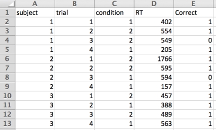
This table is formatted in the way that a lot of common psychology software (i.e. PsychoPy, Inquisit, E-Prime) records response data. From left-to-right, you can see we have three participants’ data here (1, 2, and 3 in column A), four trials for each subject (column B), two experimental conditions (C; presented in a random order), and then the actual reaction times (column D) and then a final column which codes whether the response was correct or not (1=correct, 0= error).

I created the data table using Microsoft Excel, and will do the processing with it too, however I really want to stress that Excel is definitely not the best way of doing this. It suits the present purpose because I’m doing this ‘by hand’ for the purposes of illustration. With a real data-set which might be thousands of lines long, these procedures would be much more easily accomplished by using the functions in your statistics weapon-of-choice (SPSS, R, Matlab, whatever). Needless to say, if you regularly have to deal with RT data it’s well worth putting the time into writing some general-purpose code which can be tweaked and re-used for subsequent data sets.

The procedures we’re going to follow with these data are:

1. Remove reaction times on error trials
2. Do some basic data-cleaning (removal of outlying data)
3. Re-format the data for analysis

1. Remove reaction times on error trials

As a general rule, reaction times from trials on which the participant made an error should not be used in subsequent analysis. The exceptions to this rule are some particular tasks where the error trials might be of particular interest (Go/No-Go tasks, and some others). Generally though, RTs from error trials are thought to be unreliable, since there’s an additional component process operating on error trials (i.e. whatever it was that produced the error). The easiest way of accomplishing this is to insert an additional column, and code all trials with errors as ‘0’, and all trials without an error as the original reaction time. This can be a simple IF/ELSE statement of the form:

IF (error=1) RT=RT,
ELSE RT=0

In this excel-based illustration I entered the formula: =IF(E2=1, D2,0) in cell F2, and then copied it down the rest of the column to apply to all the subsequent rows. Here’s the new data sheet:

2. Data-cleaning – Removal of outlying data

The whole topic of removing outliers from reaction time data is a fairly involved one, and difficult to illustrate with the simple example I’m using here. However, It’s a very important procedure, and something I’m going to return to in a later post, using a ‘real’ data-set. From a theoretical perspective, it’s usually desirable to remove both short and long outliers. Most people cannot push a button in response to, say, a visual stimulus in less than about 300ms, so it can be safely assumed that short RTs of, say, less than 250ms were probably initiated before the stimulus; that is, they were anticipatory. Long outliers are somewhat trickier conceptually – some tasks that involve a lot of effortful cognitive processing before a response (say a task involving doing difficult arithmetic) might have reaction times of several seconds, or even longer. However, very broadly, the mean RT for most ‘simple’ tasks tends to be around 400-700ms; this means that RTs longer than say, 1000ms might reflect some other kind of process. For instance, it might reflect the fact that the participant was bored, became distracted, temporarily forgot which button to push, etc. For these reasons then, it’s generally thought to be desirable to remove outlying reaction times from further analysis.

One (fairly simple-minded, but definitely valid) approach to removing outliers then, is to simply remove all values that fall below 250ms, or above 1000ms. This is what I’ve done in the example data-sheet in columns G and H, using simple IF statements of a similar form used for removal of the error trials:

You can see that two short RTs and one long one have been removed and recoded as 0.

3.  Re-format the data for analysis

The structure that most psychology experimental systems use for their data logging (similar to the one we’ve been using as an illustration) is not really appropriate for direct import into standard stats packages like SPSS. SPSS requires that one row on the data sheet is used for each participant, whereas we have one row-per-trial. In order to get our data in the right format we first need to sort the data, first by subject (column A), and then by condition (column C). Doing this sort procedure ensures that we know which entries in the final column are which – the first two rows of each subject’s data are always condition 1, and the second two are always condition 2:

We can then restructure the data from the final column, like so:

I’ve done this ‘by hand’ in Excel by cutting-and-pasting the values for each subject into a new sheet and using the paste-special > transpose function, however this is a stupid way of doing it – the ‘restructure’ functions in SPSS can accomplish this kind of thing very nicely. So, our condition 1 values are now in columns B:C and condition 2 values are in columns D:E. All that remains to do now would be to calculate summary statistics (means, variance, standard deviations, whatever; taking care that our 0 values are coded as missing, and not included in the calculations) for each set of columns (i.e. each condition) and perform the inferential tests of your choice (in this case, with only two within-subject conditions, it would be a paired t-test).

Next time, I’ll use a set of real reaction time data and do these procedures (and others) using SPSS, in order to illustrate some more sophisticated ways of handling outliers than just the simple high and low cutoffs detailed above.

TTFN.